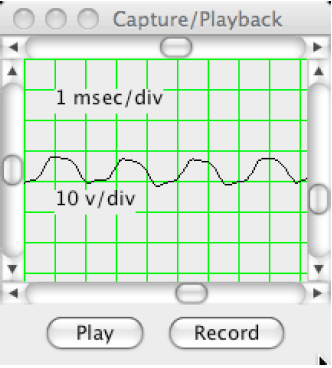
AbstractThis paper is part 5 in a series of papers about the Discrete Fourier Transform (DFT) and the Inverse Discrete Fourier Transform (IDFT). The focus of this paper is on the spectrogram. The spectrogram performs a Short-Time Fourier Transform (STFT) in order to estimate the spectrum of a signal as a function of time. The approach requires that each time segment be transformed into the frequency domain after it is windowed. Overlapping windows temporally isolate the signal by amplitude modulation with an apodizing function. The selection of overlap parameters is done on an ad-hoc basis, as is the apodizing function selection. This report is a part of project Fenestratus, from the skunk-works of DocJava, Inc. Fenestratus comes from the Latin and means, "to furnish with windows". 1 INTRODUCTION TO SHORT-TIME SPECTRAL ESTIMATIONA spectrogram (sometimes called a spectral water fall, sonogram, voiceprint or voice gram) is a visual rendering of the harmonics of an input signal as a function of time. From an implementation point-of-view, this means windowing an input signal, taking the Fourier transform and then displaying it. The window is translated in time across the signal. Window size, sample overlap, the sample rate, number of bits per-sample, etc., are application-specific design parameters. Suppose, for example, we are given a turning fork that produces a tone at 440 Hz. To compute the period of the waveform, in milliseconds, we divide 1000 by 440 Hz to obtain 2.27 milliseconds. The capture/display oscilloscope (written in Java) displays the output in Figure 1.
Figure 1. The Tuning Fork It is clear from Figure 1 that the tuning fork waveform is not sinusoidal. There are several possible reasons for this. The tuning fork is in direct contact with the microphone (it is not very loud), there is some ambient noise in the input, the digitization is only 8 bits and is using u-law coding, finally, the tuning fork waveform may not sinusoidal.
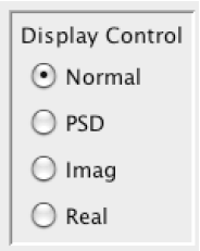
Figure 2. The Spectrogram Display Control Figure 2 shows the spectrogram display control panel. It enables the user to select a Power Spectral Density (PSD), the real part or imaginary part of the FFT or "Normal".
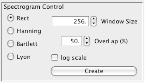
Figure 3. The Spectrogram Control Panel Figure 3 shows the control over the windowing used for the spectrogram. The window functions are described in Part 4 of this series of articles [Lyon 09]. The window size is given in samples. The log scale allows for the visualization of the subtler harmonic content of the input signal.
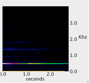
Figure 4. The Spectrogram of the Tuning Fork Without the log scale, the 440 Hz fork looks like it has 3rd harmonic content (440*3 = 1320 Hz).
Figure 5. The Spectrogram in Log Scale The log scale shows power at several harmonics (110, 220, 440, 880, 1320,and 1760). With a sample window of 256 samples and a spread of 4 KHz (at 8000 samples per second) each sample represents 4000/256 = 15.625 Hz. Further, this is not a pure tone, as the waveform suggests. To compensate, we use a 440 Hz sine wave, and compute the spectrogram.
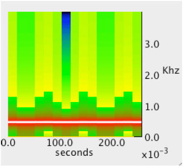
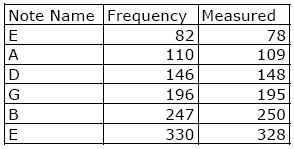
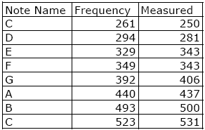
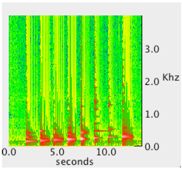
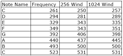
Figure 6. Spectrogram of a 440 Hz Sine Wave Figure 6 shows a log display of the PSD for a 440 Hz sine wave with a rectangular window that has 256 samples and 50% overlap. The most powerful harmonic is said to be at 437 Hz (which is only 3 Hz away from the actual 440 Hz frequency). Also, because the windows is 256 sample with an 8 KHz sampling rate, the duration of the window is 1000*256/8000 = 32 ms. This gives a reasonable frequency and temporal resolution for our voice-grade audio analyzer. The less-than-pure tone tuning fork has its two strongest harmonics at 125 Hz and 437 Hz. The 4th harmonic down from the 440 Hz signal is 110 Hz, and 125 Hz - 110 Hz is 15 Hz, which is right at the limit of the size of our 15.6 Hz bucket. An increase in the size of the window (and length of the sample) should enable an improved frequency resolution, at the expense of temporal resolution. In our last test, we increase the window size to 1024 samples. The two strongest buckets are 437 Hz and 445 Hz. This is consistent with our quantization frequency (4000 samples per second / 1024 sample = 3.9 Hz). Considering this is an old, abused tuning fork, which may not be 440 Hz, our analyzer seems to be doing pretty well. However, 1024 is a 1 second sample, and most note events do not last that long. In fact, if you average the 437 and 445 buckets together, you get 441 Hz (which is really very close to 440 Hz). 2 TUNING A GUITARGuitars are an interesting instrument for tonal identification. They can have rich harmonics (i.e., you can play chords) and they can be monophonic (i.e., they can be played just one note at a time) and they are easily tuned. I tune my guitar using the (440 Hz) tuning fork on the A string. The rest of the guitar is tuned by ear, using the fret board for relative tuning. We take the approach of playing open strings, using a 1024 sample window with 10% overlap and compare our guitar with the published turning standard for guitars [Vaughns]. Figure 7. Standard vs. Measured Frequencies Figure 7 shows the standard frequencies vs. the measured frequencies, for several note names. The nature of the guitar makes it rich in harmonics. For example, a second harmonic of G (390 Hz) is sometimes dominant in the output. Considering our predicted bucket size is 3.9 Hz, Figure 7 shows the measure frequencies to be within the bucket spread. We define the bucket spread as the center frequency +-1 bucket frequency quanta. So, 82 Hz +- 3.9 Hz is a range from 78 Hz to 86 Hz. Clearly, to reduce the bucket spread, we need more samples (either longer events or faster sample rate or both). 3 A MAJOR SCALEIn this section we play a major scale (doe re me fa sol la ti doe) and see how our analysis is able to do, based on the spectrogram. For this experiment, we use a window of 256 samples and so expect a bucket quantum of 4000/256 = 15.6 Hz. Thus showing what happens when the number of samples is too small. Figure 8. Specified and Measured Frequencies Figure 8 shows the specified and measure frequencies. Note that E and F are only 20 Hz away from one another. The mid-point frequency is only 10 Hz apart. It is clear we need more samples, or another algorithm to determine the strongest harmonic.
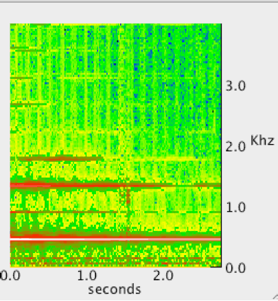
Figure 9. Spectrogram of a Major Scale Figure 9 shows the 256-sample window spectrogram. This demonstrates that, to the human eye, the E and F notes (3rd and 4th notes) are very close to one another on the graph and thus hard to tell apart. 4 INCREASING THE NUMBER OF SAMPLESThere are two ways to increase the number of samples for the signal, either increase the sample rate or increase the signal duration. In this section, we increase the signal duration to over 1 second per note, and then increase the window size to 1024 samples, with 10% overlap and a rectangular window function.
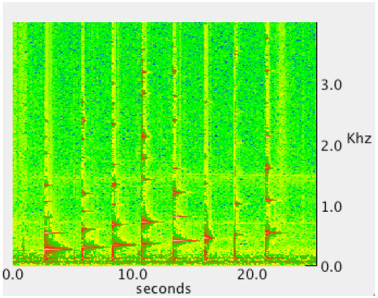
Figure 10. Long Duration Notes Figure 10 shows the spectrogram for a guitar playing the major scale, in the key of C, with notes that last for longer than 1 second. Figure 11. Comparison of 256 and 1024 Sample Windows Figure 11 shows the expected improvement in precision when the window (and signal) size increase. The ability to tell the difference between the E and the F notes has been greatly improved. The trade-off between time and frequency precision is also made far more clear. 5 SUMMARYThis paper shows how Java can be used to drive home the lesson that temporal and frequency precision are an engineering trade-off that can drive system design. Using a short-time Fourier transform, we demonstrated, both numerically and graphically, how window size, sample rate and duration impact our ability to identify pitch events on an input signal. Spectrograms are not new [Bartlett]. Nor, for that matter are the windows for doing harmonic analysis [Harris]. In fact the CMU Sphinx project has done this type of processing in the past [CMU]. However the Sphinx project used native methods. What is new is the use of Java (without any native methods) for performing this type of processing. Chris Lauer has a pure Java "Sonogram project" but this does not attempt to digitize directly from the microphone. Nor does it attempt to do note identification. There are several methods available for improving our ability to identify guitar notes. For example, each note has a unique harmonic signature. Presently, we only take the strongest harmonic. However, if we look at several harmonics, we could take advantage of individual note harmonic signatures. Extending the harmonic signature argument, we might do well to cross correlate the input signal with a bank of sampled notes, thus performing a kind of pattern recognition. The question of which approach is better remains open. REFERENCES[Bartlett] Bartlett, M. S. "Periodogram Analysis and Continuous Spectra", Biometrika 37, 1-16, 1950. [CMU] http://cmusphinx.sourceforge.net Last accessed 8/15/09. [Harris] Fredric J. Harris, "On the use of Windows for Harmonic Analysis with the Discrete Fourier Transform", Proceedings of the IEEE, V66N1, Jan. 1978, pp. 51-83. [Lauer] Chris Lauers’ Sonogram Project http://sourceforge.net/projects/sonogram/ Last accessed 8/14/09. [Lyon 09] Douglas Lyon, "The Discrete Fourier Transform: Part 4 The Spectral Leakage", Journal of Object Technology, vol. 8, no. 7, November-December 2009, pp. 23-34. http://www.jot.fm/issues/issue_2009_11/column2/ [Vaughns] "Musical Note Frequencies - Guitar and Piano" http://www.vaughns-1-pagers.com/music/musical-note-frequencies.htm Last accessed 8/14/09. About the author
Douglas A. Lyon: "The Discrete Fourier Transform, Part 5: Spectrogram", in Journal of Object Technology, vol. 9. no. 1, January - February 2010 pp. 15-24 http://www.jot.fm/issues/issue_2010_01/column2/ |
||||||||||