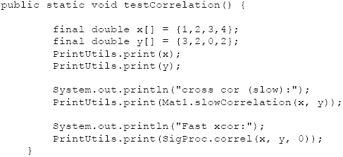
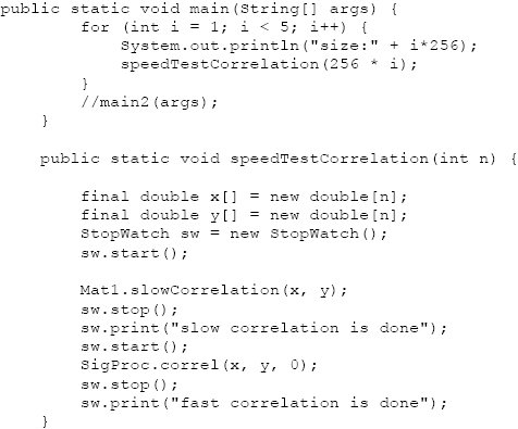
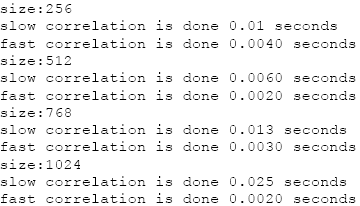
AbstractThis paper is part 6 in a series of papers about the Discrete Fourier Transform (DFT) and the Inverse Discrete Fourier Transform (IDFT). The focus of this paper is on correlation. The correlation is performed in the time domain (slow correlation) and in the frequency domain using a Short-Time Fourier Transform (STFT). When the Fourier transform is an FFT, the correlation is said to be a “fast” correlation. The approach requires that each time segment be transformed into the frequency domain after it is windowed. Overlapping windows temporally isolate the signal by amplitude modulation with an apodizing function. The selection of overlap parameters is done on an ad-hoc basis, as is the apodizing function selection. This report is a part of project Fenestratus, from the skunk-works of DocJava, Inc. Fenestratus comes from the Latin and means, “to furnish with windows”.1 INTORDUCTION TO CROSS-CORRELATIONCross-Correlation (also called cross-covariance) between two input signals is a kind of template matching. Cross-correlation can be done in any number of dimensions. For the purpose of this presentation, we define one-dimensional normalized cross-correlation between two input signals as: The coefficient, r, is a measurement of the size and direction of the linear relationship between variables x and y. If these variables move together, where they both rise at an identical rate, then r = +1. If the other variable does not budge, then r = 0. If the other variable falls at an identical rate, then r = -1. If r is greater than zero, we have positive correlation. If r is less than zero, we have negative correlation. When (1) is computed, for all delays, then the output is twice that of the input. It is common to use the pentagon notation when showing a cross correlation: Where the asterisk indicates the complex conjugate (a negation of the imaginary part of the number). Input signals should either have the same length, or there should be a policy in place to make them the same (perhaps by zero padding or data replication). If the input signals are real-valued, then we can write: Comparing (4) with the convolution: Shows that Y is time-reversed before shifting by n. In comparison, correlation has shifting without the time reversal. 2 AN EXAMPLE, IN EXCELSuppose you are given two signals that have already had their means subtracted. Correlate the signals, without dividing by the standard deviation. The signals are: X=1,2,3,4 with Y = 3, 2, 0, 1.
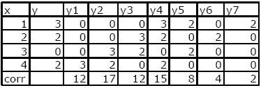
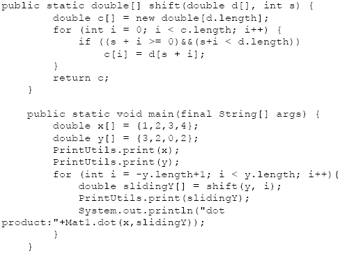
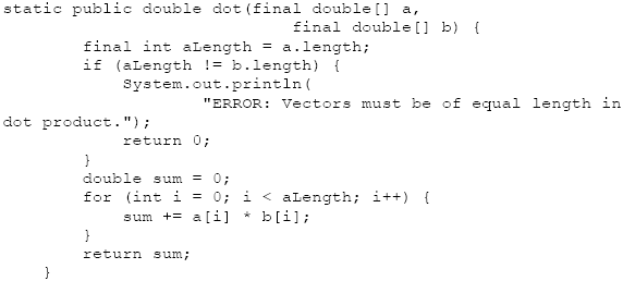
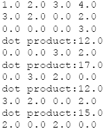
Figure 1. Y is shifted 7 times Figure 1 demonstrates that a moving cross correlation requires that the kernel of the signal be shifted so that its leading edge appears and then is shifted until only the trailing edge can be seen. After each shift, the rest of the signal is padded with zeros. The row labeled corr contains the correlation and results from the dot product of X with Y. For example X•Y1=12, X•Y2=17, etc. 3 A SLOW CROSS CORRELATIONWe implement the slow cross correlation using a sliding dot product: Where the dot product is implemented using: The output matches that given in Figure 1: The implementation is clearly not optimized, but it is correct and serves to illustrate the sliding dot product nature of the cross correlation. 4 A FAST CORRELATIONA slow implementation of the moving cross correlation algorithm, as shown in Figure 1, will take O(N**2) time. Further, the unoptimized implementation, shown in section 3, has high constant time overhead. Using the FFT and the correlation theorem, we accelerate the correlation computation. The correlation theorem says that multiplying the Fourier transform of one function by the complex conjugate of the Fourier transform of the other gives the Fourier transform of their correlation. That is, take both signals into the frequency domain, form the complex conjugate of one of the signals, multiply, then take the inverse Fourier transform. This is expressed by: We now compare the slow correlation with the fast correlation: The output follows: The fast correlation makes use of the FFT, and gets identical results to the slow correlation. So how much faster is the FFT than the slow correlation for small sized arrays? The testing code follows: Even for modest arrays, we see substantial speedup (between 2.5 and 12 times faster, for small array sizes): 5 SUMMARYThis paper shows how the FFT can be used to speed up cross correlation. Further, it shows that even for small array sizes, substantial speed up can be obtained by using the fast cross correlation. Arguments for using the FFT to accelerate the cross correlation are often not supported with specific data on computation time (a situation, which this paper remedies) [Lyon 97]. The cross correlation has uses in many fields of scientific endeavor (music, identification of blood flow, astronomical event processing, speech processing, pattern recognition, financial engineering, etc.). One of the basic problems with the term normalization when applied to the cross-correlation is that it is defined in different places differently. For example, Pratt suggests that the number of elements in the normalization (an even a square root) is not needed [Pratt]. Lewis suggests using both the square root and the average [Lewis]. Therefore the question of which normalization to use is application-specific. REFERENCES[Lewis] “Fast Normalized Cross-Correlation” by J.P. Lewis, http://www.idiom.com/~zilla/Papers/nvisionInterface/nip.html last accessed 8/24/09. [Lyon 97] Java Digital Signal Processing, Douglas A. Lyon and H. Rao, M&T Press (an imprint of Henry Holt). November 1997. [Pratt] W. Pratt, Digital Image Processing, John Wiley, New York, 1978. About the author
Douglas A. Lyon: “The Discrete Fourier Transform, Part 6: Cross-Correlation”, in Journal of Object Technology, vol. 9. no. 2, March - April 2010 pp. 17 - 22 http://www.jot.fm/issues/issue_2010_03/column2/ |
||||||||||

